Using macros to model

Modelling a Plunger

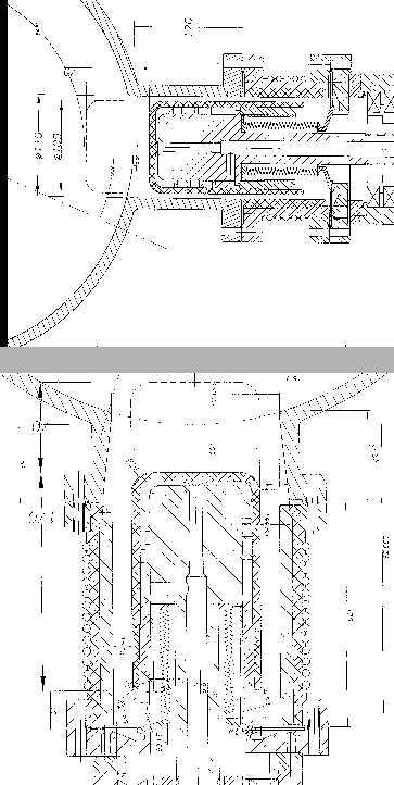
Both plungers are topologically the same. They consist of a tube where inside of the tube a circular cylinder with a rounded cap sits in.

Figure 5.2: Details of the technical drawing, showing the plungers.

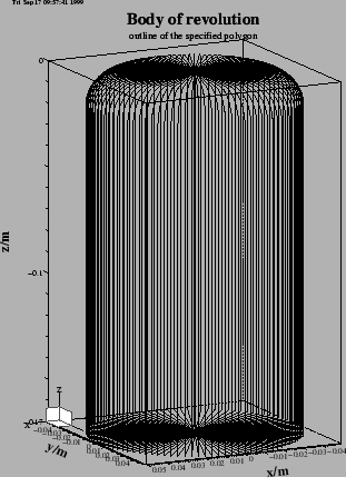
Figure 5.3: An outline of the body of revolution that shall decribe the body of a plunger.

A plunger is a body of revolution. gd1 can model this directly. We edit our inputfile so that it contains:

 #
 # a plunger
 #
 define(PlungerRadius0, eval(110e-3/2) )
 define(PlungerInnerRadius, eval(100e-3/2) )
 define(PlungerCurvature, 16e-3)

 -gbor
     material= 10
     originprime= (0,0,0)
     zprimedirection= (0,0,1)
     rprimedirection= (1,0,0)
     range= (0,360)

     clear
        # point= (z,r)
     point= (0,0)
     point= (0, eval(PlungerInnerRadius-PlungerCurvature) )
        arc, radius= PlungerCurvature, size= small, type= counterclockwise
     point= (eval(-PlungerCurvature), PlungerInnerRadius)
     point= (-170e-3, PlungerInnerRadius)
     point= (-170e-3, 0 )
 show= now,
     doit

The figure 5.3 shows an outline of the body of revolution that this decribes. This plunger has its axis direction in z-direction. Our plungers shall have their axis lying in the x-y-plane, with an angle of -90+22.5 and 17 degrees. In order to have the axis of our plunger direct in the proper direction, we change the values of zprimedirection, rprimedirection. These two vectors define the local z', r' coordinate-system, in which the body of revolution is described. We edit our inputfile:

 define(PlungerAngle, eval((-90+22.5)*@pi/180))
     originprime= (0,0,0)
     zprimedirection= (eval(-cos(PlungerAngle)),\
                       eval(-sin(PlungerAngle)),\
                       0)
     rprimedirection= (0,0,1)

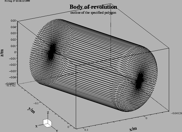
The resulting outline is shown in figure 5.4.

Figure 5.4: The plunger now has its axis showing in the right direction.

We are not done yet: The plunger is not yet at the right position. The origin of the plunger shall not be at (x,y,z)=(0,0,0), but at (x,y,z)=( $r \cos(\varphi), r \sin(\varphi), 0$), with $\varphi = -90+25$ degrees. We change our inputfile:

 define(PlungerRadius0, eval(OuterRadius-50e-3))
 define(PlungerAngle, eval((-90+22.5)*@pi/180))
     originprime= (eval(cos(PlungerAngle)*PlungerRadius0),\
                   eval(sin(PlungerAngle)*PlungerRadius0),\
                   0)
     zprimedirection= (eval(-cos(PlungerAngle)),\
                       eval(-sin(PlungerAngle)),\
                       0)
     rprimedirection= (0,0,1)

When we feed gd1 with this inputfile, we do not see the plunger in the plot of the material-discretisation. The reason is: The plunger is outside of the specified computational volume. Since the geometry with the plunger does no longer have all three symmetry-planes, we have to compute in a much larger volume. The only symmetry plane left is the plane z=0. So we change the specifications for the boundaries of the computationals volume to:

 ###
 ### We define the borders of the computational volume,
 ### we define the default mesh-spacing,
 ### and we define the conditions at the borders:
 ###
 -mesh
     spacing= eval(InnerRadius/15)
     pxlow= eval(-1.1*OuterRadius)
     pylow= eval(-1.1*OuterRadius)
     pzlow = eval(-(GapLength/2+TaperLength+9e-2))
     pxhigh= eval( 1.1*OuterRadius)
     pyhigh= eval( 1.1*OuterRadius)
     pzhigh= 0

     #
     # The conditions to use at the borders of the computational volume:
     #
     cxlow= electric, cxhigh= electric
     cylow= electric, cyhigh= electric
     czlow= electric, czhigh= electric

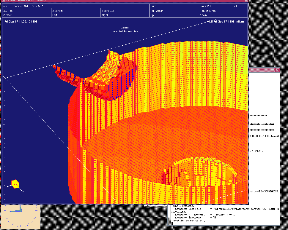
The so edited inputfile can be found as "/usr/local/gd1/Tutorial-SRRC/wPlunger00.gdf". When we feed gd1 with this inputfile (gd1 $<$ wPlunger00.gdf), we see a picture similiar as the one shown in figure 5.5

Figure 5.5: Screenshot of the desktop when the inputfile wPlunger00.gdf has been fed into gd1.

Using macros to model