Computing Wakepotentials

Voltages at different paths : How to steer gd1.pp from a shell script

Our structure so far is a purely rotational symmetric one. Therefore, if the geometry would have been modelled perfectly, the shunt-impedance (for the monopole mode) at other locations (x,y)^3.1 should be exactly the same^3.2 as the shunt-impedance at (x,y)=(0,0). We now use this property of rotational symmetric structures to estimate the discretisation error we have to live with.

It suffices to compute the voltage at different paths, the stored energy of course is independent of the position (x,y). We compute the voltages at all positions (xi,0) and (0,yi) that are available in the grid. These positions of the grid planes are available in gd1.pp as the symbolic functions @x(i), @y(i), @z(i). The total number of grid planes are available as @nx, @ny, @nz. These symbols are only available after a database has been specified in -general.

So, to compute the voltages at all possible positions (xi,0) we may say:

 -lintegral
    symbol= e_1
    direction= z, component= z
    do ix= 1, @nx
       startpoint= ( @x(ix), 0, @zmin )
       doit
       echo voltage along ( @x0 , @y0 , z=z ) is @vreal @vimag @vabs
    enddo

If we do this, we get a lot of messages on the screen. In order to have a nice graphic of the dependence of the voltage on x, we better redirect the output to a file and process the result slightly. We write a small shell script:

#!/bin/sh

 #
 # feed the postprocessor with a 'here'-document,
 # 'tee' the output of the postprocessor to the file "pp.out"
 #

 (gd1.pp | tee pp.out) << EOF

    nomenu, noprompt, nomessage     # no unneccessary output
    -general, infile= @last
    -lintegral
       symbol= e_1
       direction= z, component= z
       do ix= 1, @nx
          startpoint= ( @x(ix), 0, @zmin )
          doit
          echo @x0 @vreal @vimag # <= x, vreal, vimag
       enddo
    end
EOF

 #
 # Write a PlotMtv-header to "x-voltages.mtv".
 #
 # Process the file "pp.out":
 # 'grep' the lines with the pattern "vreal"
 #
 echo \$ DATA= COLUMN  >  x-voltages.mtv
 echo x vreal  vimag   >> x-voltages.mtv

 grep vreal pp.out     >> x-voltages.mtv

 #
 # now start "mymtv2" to display the data:
 #
 mymtv2 -mult -landscape x-voltages.mtv

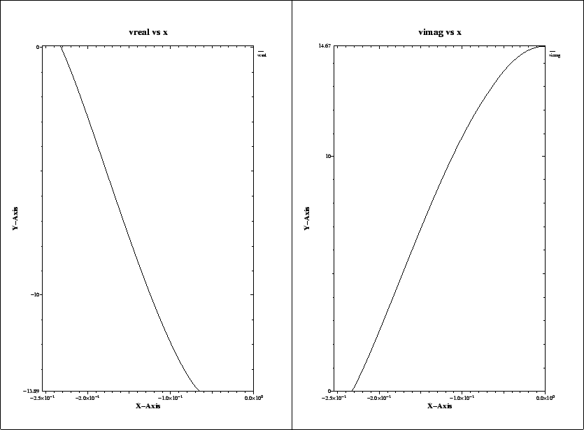
3.4 This shell-script can be found as "/usr/local/gd1/Tutorial-SRRC/x-voltages.x". The resulting plot is shown in figure 3.4. We see that the real part of the integrated voltage is almost constant in the range $\vert x\vert < 0.065$m. The value of 0.065 m is the radius of the entrance of the cavity. The imaginary part is not constant, but it would be, if we would have modelled the full z-length of the geometry (it would be zero then).

Figure 3.4: The real part and imaginary part of the integrated voltage as a function of the position x. This plot has not been generated directly by gd1.pp, but has been produced by a simple shell-script.

Footnotes

... (x,y)^3.1

The locations (x,y) where the shunt impedance has to be the same are the locations where a beam can travel.

... same^3.2

That the shunt-impedance for the monopole mode has to be constant follows from the Panofsky-Wenzel theorem.

Computing Wakepotentials